Magic of a VLookup with Match: A Complete Guide

Welcome to this article on the most loved and used excel formulas- VLOOKUP (Vertical Lookup) in combination with MATCH which helps to find out the information between two or multiple tables. This is the most used formula in excel and in fact on other analytics tools also , for e.g., in VBA, Python, Power Query, Power BI, Databases (Access, SQL Server) this function do exists.

However, important point to note is that VLookup is known by a different name on few data analytics Tools. For example, in databases, it is called Joins, in Power Query it is available as a Merge feature, in python too it is called a merge function. This is just for your extra knowledge. No charges for this extra knowledge😊😊.

If you are a beginner and want to deep dive into VLOOKUP, MATCH functions and their combinations, you are at the right page. I bet, you will not stop smiling after completing this article.

Topics we are going to cover:

What is VLookup – Vertical Lookup?
Find the Exact match with VLookup.
Find the Approximate match with VLookup.
VLookup with Multiple Criterias ( It’s Awesome )
How to make VLookup dynamic ( Intro to Mr Match function 😁 )
What is a Match Function?
How to use Nested VLookup (To make you a Super man in excel )
Errors you may see while working with VLookup (Be a Strong in fundamentals )
Limitations of VLookup ( Even we have limitations .😁 Limitations means challenges and challenges mean Inventions )

1.) What is a VLookup?

Vlookup is a vertical lookup which is primarily used to find and retrieve information from a specific column within a table. It searches for a given value in the leftmost column of a table and returns a corresponding value from a specified column in the same row.

Vlookup enables you to retrieve the required information in just a few clicks instead of finding information manually through rows and columns. This formula seems interesting right as it’s saving our precious time and effort.

So, let’s dive further to learn more about it.

Syntax and Parameters of Vlookup:

To master the vlookup it’s important to learn its syntax and parameters. Let’s break down Vlookup and explore each element in detail.

The Syntax of Vlookup formula consist of following:

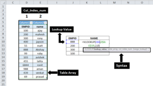
=VLOOKUP(lookup value,table array,column index number,range lookup)

So As we can see Vlookup has four parameters which are 1. lookup Value, 2.table array, 3.column index numbers and 4.range lookup.

Let’s understand what does this parameter means:

Lookup Value: This specifies the value which you want to search or lookup in the data.
Table Array: This specifies the cell range containing the lookup value and the value you want as output. Please note that the lookup value must be in the first column in the given range. For example, if your lookup value is in cell A5, then your range should start from column A.
Column Index Number: This specifies the column number in the given range contains the value you want the vlookup to return.Column index number tells excel from which column the data should be retrieved.let’s take an example, if your table array is A1:B15, Column A will be your 1st column and Column B will your 2nd column.
Range Lookup: It has two options i.e. True and False. True will return the approximate match and False will return the exact match. By default, vlookup always returns an approximate match(which is a True option). If you want an exact match then select the False option and Most of the time we always use the exact match. We can also enter 0 for exact match and 1 for approximate match, which we will see in the coming examples.

So excited for the next section? We will understand how to use the VLookup.

2. Find the Exact match in Vlookup:

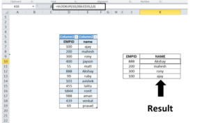
So let’s take the above picture as an example. We have an employee ID and Employee Name table as data and we have to find the employee name from the given table in cell K10 to K13 . As you can see in cell K10, we have used the Vlookup formula to find the output from a given table. The formula used is =Vlookup(J10,D$6:E$19,2,0). Now, Let’s see the parameter from the formula in detail.

Always remember to use “=” Sign before any formula in excel to get a result.

In the first parameter, we have taken Cell J10 as a lookup value we want to search for.
In the second parameter, We have specified the table which contains the lookup value and output value. We took the table location D$6:E$19. Please be noted that we have used $ sign for the absolute reference so that we can copy the formula to the next row. We have also discussed this part in our video.
In the third parameter, we have entered 2 as a column index number. It will return the output value that we are looking for from the second column.
In the last parameter, we have entered 0 for the exact match. We can also use FALSE which also means 0 in excel. Just give it a try. Go in excel cell and type FALSE and press enter. Now , go to in other cell and type = 1* that cell where you have written FALSE(for e.g. =1*A1). You may be thinking, why we are multiplying FALSE with 1 because it is a text value and lead to an error. Surprisingly, you shall see not an error but a value which is 0. Reason is FALSE in excel is not treated as a text. It is a number and it has a zero value. Similarly, If you write TRUE in excel cell and try to multiply that with any number , you will see the same result back into the cell because excel treats TRUE as a number 1. Yes, you heard me right. TRUE is 1 and FALSE is 0 in excel world. Just do it. Have fun with this.

So, if Lookup is not found in the table, It will return an N/A value provided formula is correctly written with all the dollar signs in formula, wherever applicable

Below is the result with the exact match of VLookup. As we can see VLookup given the value as result is the same with the given table.

3. Find the Approximate Match in VLookup:

Approximate match is default range lookup in VLookup formula. If we do not give any instruction in range lookup, excel assumes range lookup to an approximate match.

Approximate match is used less frequently as compared to exact match in most of the cases. If the lookup value is not available in the table array then an approximate match is useful to get the result. If Empid 100 is not found in a table, approx match starts finding the smaller number than 100 w🤣🤣whichever is a closest value. Exact match does not look for any close match. It immediately says -sorry not found.

Please note that in order to get the correct result in approximate match it is very necessary to sort the first column of the range data either numerically or alphabetically.

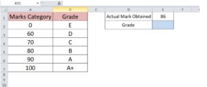
Let’s understand the Approximate match with an example. Suppose, we have the following dataset of students’ grades in the image below and we have to find the students’ grades based on actual marks obtained. As we can see the value 86 as actual mark obtained is not in the given table.

Now, we will use a VLookup with an approximate match to find the results.

We have used the VLookup formula as followed:

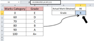
=VLOOKUP(E1,A1:B7,2,1)

In the formula our first parameter is Cell E1 which is lookup value, A1:B7 is second parameter as table array, In third parameter we selected 2 as our required output is in the second column of the table and in the forth parameter we have entered 1 as range lookup. We can also enter TRUE instead of 1 as both will bring an approximate match in Vlookup. Then, Vlookup has given Value “B” as an output and Vlookup gives closed match as output in approximate match. You see 86 is not available in a table. Correct! Now, because of approx match, Vlookup will find out the closest number to 86 but it has to be a smaller than 86. So, it is 80 and that is why we see Grade B. I am again reiterating , that main table has to be sorted in asc order otherwise it will lead to wrong results. This is a condition in Vlookup so we have to fulfil it without forgetting it. Hope, now you have no doubt about exact and approx match parameters. So, you see approx match has its own importance. Sometimes, you desperately needs it.

4. VLookup with Multiple Criteria:

The Vlookup function does not handle multiple criteria or more than one lookup value genetically but we can have a control on it. We can use a helper column to join multiple fields together and we can use a helper column to bring our result. It seems interesting, right? Lets see in the example below.

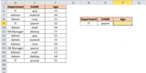
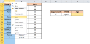
As we have Department, Name and Age data in the table shown in above image and we have to lookup the Age of Jayson in the IT department. But as Name and Department are in two different columns, we will add a helper column which will store combined values of both columns. We can add click on column header and click on insert.

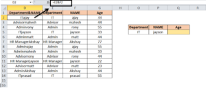
This will add the column at left of the department column, let’s give it name by “department&Name”. We will combine the department and Name column by using =E2&F2 formula below the header of the “E” column and we will drag the formula down.

Now that we successfully created the helper column, we can now look up for the value and find our output in the Q5 cell using Vlookup as shown in below image.

We have used the formula as follows:

=VLOOKUP(O5&P5,D1:G14,4,0)

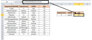
In the first parameter we have combined the Cell O5 and P5 to get our lookup value to lookup in the helper column. We have used the ”&” function to join cells and instead of “&” function we can also use the concatenate function i.e CONCATENATE(O5,P5). The second parameter is the table range D1:G14. The third parameter specifies the column index number as the output is in the 4th column. The fourth parameter is 0 to get an exact match and As you can see in the above image that VLookup has given 33 as output.

5. How to make VLookup dynamic (Bring Mr Match function here):

Well, Vlookup is one of the most popular functions but when you will explore it more, you will realize that vlookup is not the dynamic formula which is one of its problems.

In Vlookup, column index number is a static value hence vlookup doesn’t work as a dynamic formula. Also if you have multiple column data it’s very time consuming to change its reference manually. But VLookup with a match function combined can solve this problem.

Let’s explore it more with an example for better understanding.

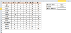
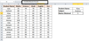
As you can see in the above picture, we have a table of Students Name, Subject and its marks obtained. Now you have to find Marks obtained for Vijay in science subject.

The formula should be like this to get output :

=VLOOKUP(I2,A1:F14,3,0)

In this formula we have taken Cell I2 as lookup values i.e. Vijay. The table array is A1:F14. We have taken 3 as a column index number as the output is in the 3rd column of the table with header “science” and entered 0 for an exact match.

But suppose your boss tells you to get marks for Hindi Subject. You will need to change the value in Col_index_num as 4 as Hindi is the 4th column. Because it is not dynamic.

So to make Vlookup dynamic, the best way is to replace it with the Match function.

6. MATCH Function :

So first let’s understand what the match function is and how it works.

Match function is similar to Vlookup but only difference is that match function gives the cell number of lookup value in row or column. Match function finds the cell position of the lookup value from the table range. It means Vlookup can return a boolean, text, number, decimal value as an output but match only returns a number value because position is always a number. It is not text or decimal. 😊😊

Syntax of Match is as followed:

=MATCH(lookup_value,lookup_array,[match_type])

Match function has three parameters. First is lookup_value means the value which we are finding, second is lookup_array means a range or Table to lookup the value and third is match type to specify the approximate match or exact match. You see, this last parameter is same as in Vlookup function.

Exact match : If I have to find out the position of an “apple” in a main table.It is going to return the position of an apple.

Now, the question is how approximate is going to work? I mean, How do you find the approximate match of an apple. 🤣🤣🤣. You know we have learnt in Vlookup function, approximate means find out the nearest value of an lookup and it must be shorter value than lookup. If i am using a Vlookup function and checks the name of ID 100 , If id is not available in the main table, approximate finds out the nearest value to 100 and at the same time it should be lesser than 100 like it can be 99,98 ,97 or whatever. The most nearest value.This principal of Vlookup works the same way in Match too. So, it means , if i have to find out the position of 100 id in main table and it is not found then approximate in match finds out the nearest matches.

So,Approximate match never works on text values ,in both functions because in text, we cannot find out the nearest matches. It is a common sense thing. At the same time, in both functions, I have mentioned this before too, your main table must be sorted in ascending order otherwise results will be wrong.

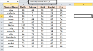
Let’s take the example to understand it well. In the image below I have lookup the name “Science” with the match function from a heading row.

And it has returned the value 3 as the name is in the third cell of the header row.

Now that you know how the match function works, Let’s continue with our previous example and put the Vlookup and Match together.

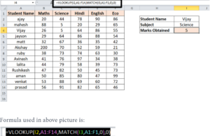
In the above picture we have used the vlookup formula to lookup value for “Vijay” and for col_index_num we have used the Match function instead of any static value. Also in the Match function we have used “Science” as a lookup value and the Match function has returned the cell number of the “Science” from the given range. Then vlookup has taken that cell number as col_index_num to get the output .Basically, Match function tells vlookup the column number to get the required result.

And now you don’t need to change the column number manually, let’s take another example. We will just change the student name to “Akshay” and subject name to “English” and we will keep the formula in cell I4 as it is. Let’s see what results we get in the picture below.

So, As you can see we just changed the student name and Subject without changing the formula in cell I5 and We have got the result we want. Problem Solved!!!

7. How to use Nested VLookups?

Hopefully, we must have become familiar with the Vlookup function by reading this article till here, let’s see another beauty of the Vlookup function to save our time and space. We will cover Nested Vlookup here.

It is nothing but nesting the Vlookup function together as per the need. Sometimes you may need to lookup the value which is interlinked with different tables so instead of using a separate Vlookup function for each value we can nest the Vlookup function together and find our output in one go.

Let’s see an example to understand it well.

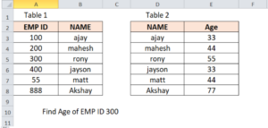
As we can see in the above picture we have two tables. First table has Emp ID and Name data and the second table has employee name and Age data. Just for an easy view I have added the same table closer but you may have a case that both tables would be in different sheets. However, the steps applied for both will be the same. Now as shown in the above picture we have to find the Age with a lookup value as EMP ID. Now, you may use two separate formulas to find the result as shown below.

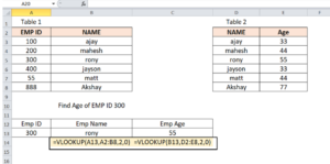
As we can see in the above picture the Age can be found by using two separate Vlookup.

The first formula which is =VLOOKUP(A13,A2:B8,2,0) has extract the “Rony” as Name from Table 1, and by applying Vlookup in next cell on employee name as lookup value on Table 2, Vlookup has given the Age as result. It looks simple but it’s taking the extra space in excel, however by combining the vlookup we can directly get the Age in one go. All we have to do is nest the first vlookup formula inside the input of the second Vlookup formula. And believe me, the process is very simple. Let’s see in the picture below.

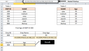
By doing nesting of Vlookup the formula will look like this:

In the Vlookup formula of above picture, The inner vlookup looks for EMP ID and returns the Name and outer vlookup takes the inner vlookup output as its lookup value i.e. Name and return the Age from table 2.

Nested Vlookup is very useful when you have multiple sheets and complex tables. And the best thing about this is you can keep nesting Vlookup as much as you want. It saves several steps and also avoids a lot of confusion.

8. Errors you may face in VLookup:

There are few common issues due to which VLookup can throw the below errors.

i.) #N/A – Not available

- Lookup value does not exist in the leftmost column of the table array.
- Extra Spaces in lookup value – Sometimes it could be the reason for the error, which we can investigate if vlookup gives an error and remove the space to get a result.
- Mistakes in the lookup typo – We could get this if there is a typo mistake in lookup value as Vlookup cannot give the result to wrong lookup value. Suppose, you have aple in your table and in main table it is correctly spelled as apple. That can also be a reason. Just correct the typo.

ii) #REF! – Reference Error

- It can give this error when we have entered the table range that does not exist.
- It can also give an error when we have entered a column index number which is greater than columns present in the table.

iii) #VALUE! – Value Error

- This error can occur when column index number values entered less than 1 or not a numeric value. For example, Column index refers to the position of a header that you are finding it out. Correct! For eg. I want to find out empid 100 age in the table so here age is a header and i have to see the position of an age in the main table. So, if i enter position as -1 it does not make sense. It has to be 1,2,3 or whatever ,depending on the position of age header. Are you with me ? Understood? So, this error can come. Same way , column index cannot be a text.

9.) Limitations in VLookup:

As we have discussed the power of Vlookup, but like any tool it also has some limitations. Let’s see its limitations in detail.

Vlookup only searches the output form left to right direction. No support in reverse direction :

It’s one of the main drawbacks of vlookup that it can only look at the columns which are right side of the lookup value.

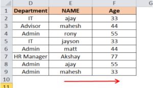
In the above image, we have the data of employees Department, Name and Age. but suppose I want to extract the Department using Name as a lookup value. Vlookup cannot give the output the only column we can extract is Age by using the Name as lookup value as the Age column is at the right side of the Name column. In order to extract the department , the Name column should be at the first column of the table.

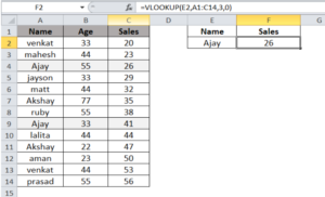
a. Vlookup can only find the first match:

In your table data if you have duplicate values in the lookup column then VLookup only extracts the result of the first lookup value.

As we can see in the above picture, we have the data of sales of the employees. In cell F2 we have used the vlookup formula to find the sales of Ajay, But we have two entries of the Ajay in the given table and vlookup has given the sales of first Ajay which is 26. It cannot give the value as output for the next entry of Ajay.

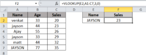
b. VLookup is not a case sensitive: (in fact whole excel including VBA is a case-insensitive- actually its not a limitation but some thinks that way)

VLookup has one of its limitations that it cannot distinguish between the lowercase and uppercase values. VLookup considers them as the same. I personally find this a good feature because I don’t like the sensitivity concept like we have in powerquery and python languages. But, it does not matter. it is just a matter of choice.

As we can see in the above picture, we have the data of sales of employees. In the F2 cell I want to extract the sales for the JAYSON which is the last row of the table but there is another jayson name in the table with different sales. And as vlookup cannot distinguish between the Uppercase and Lowercase hence the value in F2 cell extracted for jayson.

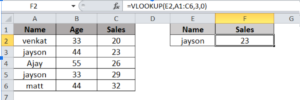
c. Inserting a new column will give incorrect results.

Vlookup gives the incorrect results if you add any new column into the lookup table when we enter the col_index_num manually.

Let’s see an example.

In the above picture, we have used the VLookup formula in cell F2 to find the sales of jayson. We have entered the column index number as 3 as our output value is in the 3rd column. But let’s add a column in the table and see.

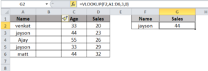
Now I have added an extra column after the Name column. Vlookup in Cell F2 has extracted the output as 44 which is from the Age column, it’s just because Vlookup is looking the output in the third column and to get the correct result we would have to manually change the column index number to 4.

Please remember, these are limitations but you know we can always work out on these limitations either by correcting the things or by introducing the functions like XLOOKUP or INDEX. I will cover these functions in another article. For e.g. , INDEX and XLOOKUP can work in any direction and lookup position does not matter unlike in VLOOKUP Case. One thing if we know sooner which is that no single function can do the job in excel. It is all about combinations of formulas , creating helper columns or rows.

Hope, you have liked the article because I have tried best to give you the best knowledge. Someone left a comment that blog is better than a book. I was flying in the air when i read that.❤️❤️❤️ Thank you so much. See you in another article.

If you are a beginner and want to deep dive into VLOOKUP, MATCH functions and their combinations, you are at the right page. I bet, you will not stop smiling after completing this article.

Topics we are going to cover:

What is VLookup – Vertical Lookup?

Find the Exact match with VLookup.

Find the Approximate match with VLookup.

VLookup with Multiple Criterias ( It’s Awesome )

How to make VLookup dynamic ( Intro to Mr Match function 😁 )

What is a Match Function?

How to use Nested VLookup (To make you a Super man in excel )

Errors you may see while working with VLookup (Be a Strong in fundamentals )

Limitations of VLookup ( Even we have limitations .😁 Limitations means challenges and challenges mean Inventions )

1.) What is a VLookup?

Vlookup is a vertical lookup which is primarily used to find and retrieve information from a specific column within a table. It searches for a given value in the leftmost column of a table and returns a corresponding value from a specified column in the same row.

Vlookup enables you to retrieve the required information in just a few clicks instead of finding information manually through rows and columns. This formula seems interesting right as it’s saving our precious time and effort.

So, let’s dive further to learn more about it.

Syntax and Parameters of Vlookup:

To master the vlookup it’s important to learn its syntax and parameters. Let’s break down Vlookup and explore each element in detail.

The Syntax of Vlookup formula consist of following:

=VLOOKUP(lookup value,table array,column index number,range lookup)

So As we can see Vlookup has four parameters which are 1. lookup Value, 2.table array, 3.column index numbers and 4.range lookup.

Let’s understand what does this parameter means:

Lookup Value: This specifies the value which you want to search or lookup in the data.

Table Array: This specifies the cell range containing the lookup value and the value you want as output. Please note that the lookup value must be in the first column in the given range. For example, if your lookup value is in cell A5, then your range should start from column A.

So excited for the next section? We will understand how to use the VLookup.

2. Find the Exact match in Vlookup:

Always remember to use “=” Sign before any formula in excel to get a result.

In the first parameter, we have taken Cell J10 as a lookup value we want to search for.

In the third parameter, we have entered 2 as a column index number. It will return the output value that we are looking for from the second column.

So, if Lookup is not found in the table, It will return an N/A value provided formula is correctly written with all the dollar signs in formula, wherever applicable

Below is the result with the exact match of VLookup. As we can see VLookup given the value as result is the same with the given table.

3. Find the Approximate Match in VLookup:

Approximate match is default range lookup in VLookup formula. If we do not give any instruction in range lookup, excel assumes range lookup to an approximate match.

Please note that in order to get the correct result in approximate match it is very necessary to sort the first column of the range data either numerically or alphabetically.

Let’s understand the Approximate match with an example. Suppose, we have the following dataset of students’ grades in the image below and we have to find the students’ grades based on actual marks obtained. As we can see the value 86 as actual mark obtained is not in the given table.

Now, we will use a VLookup with an approximate match to find the results.

We have used the VLookup formula as followed:

=VLOOKUP(E1,A1:B7,2,1)

4. VLookup with Multiple Criteria:

This will add the column at left of the department column, let’s give it name by “department&Name”. We will combine the department and Name column by using =E2&F2 formula below the header of the “E” column and we will drag the formula down.

Now that we successfully created the helper column, we can now look up for the value and find our output in the Q5 cell using Vlookup as shown in below image.

We have used the formula as follows:

=VLOOKUP(O5&P5,D1:G14,4,0)

5. How to make VLookup dynamic (Bring Mr Match function here):

Well, Vlookup is one of the most popular functions but when you will explore it more, you will realize that vlookup is not the dynamic formula which is one of its problems.

In Vlookup, column index number is a static value hence vlookup doesn’t work as a dynamic formula. Also if you have multiple column data it’s very time consuming to change its reference manually. But VLookup with a match function combined can solve this problem.

Let’s explore it more with an example for better understanding.

As you can see in the above picture, we have a table of Students Name, Subject and its marks obtained. Now you have to find Marks obtained for Vijay in science subject.

The formula should be like this to get output :

=VLOOKUP(I2,A1:F14,3,0)

In this formula we have taken Cell I2 as lookup values i.e. Vijay. The table array is A1:F14. We have taken 3 as a column index number as the output is in the 3rd column of the table with header “science” and entered 0 for an exact match.

But suppose your boss tells you to get marks for Hindi Subject. You will need to change the value in Col_index_num as 4 as Hindi is the 4th column. Because it is not dynamic.

So to make Vlookup dynamic, the best way is to replace it with the Match function.

6. MATCH Function :

So first let’s understand what the match function is and how it works.

Syntax of Match is as followed:

=MATCH(lookup_value,lookup_array,[match_type])

Match function has three parameters. First is lookup_value means the value which we are finding, second is lookup_array means a range or Table to lookup the value and third is match type to specify the approximate match or exact match. You see, this last parameter is same as in Vlookup function.

Exact match : If I have to find out the position of an “apple” in a main table.It is going to return the position of an apple.

Let’s take the example to understand it well. In the image below I have lookup the name “Science” with the match function from a heading row.

And it has returned the value 3 as the name is in the third cell of the header row.

Now that you know how the match function works, Let’s continue with our previous example and put the Vlookup and Match together.

And now you don’t need to change the column number manually, let’s take another example. We will just change the student name to “Akshay” and subject name to “English” and we will keep the formula in cell I4 as it is. Let’s see what results we get in the picture below.

So, As you can see we just changed the student name and Subject without changing the formula in cell I5 and We have got the result we want. Problem Solved!!!

7. How to use Nested VLookups?

Hopefully, we must have become familiar with the Vlookup function by reading this article till here, let’s see another beauty of the Vlookup function to save our time and space. We will cover Nested Vlookup here.

It is nothing but nesting the Vlookup function together as per the need. Sometimes you may need to lookup the value which is interlinked with different tables so instead of using a separate Vlookup function for each value we can nest the Vlookup function together and find our output in one go.

Let’s see an example to understand it well.

As we can see in the above picture the Age can be found by using two separate Vlookup.

By doing nesting of Vlookup the formula will look like this:

In the Vlookup formula of above picture, The inner vlookup looks for EMP ID and returns the Name and outer vlookup takes the inner vlookup output as its lookup value i.e. Name and return the Age from table 2.

Nested Vlookup is very useful when you have multiple sheets and complex tables. And the best thing about this is you can keep nesting Vlookup as much as you want. It saves several steps and also avoids a lot of confusion.

8. Errors you may face in VLookup:

There are few common issues due to which VLookup can throw the below errors.

i.) #N/A – Not available

Lookup value does not exist in the leftmost column of the table array.

Extra Spaces in lookup value – Sometimes it could be the reason for the error, which we can investigate if vlookup gives an error and remove the space to get a result.

Mistakes in the lookup typo – We could get this if there is a typo mistake in lookup value as Vlookup cannot give the result to wrong lookup value. Suppose, you have aple in your table and in main table it is correctly spelled as apple. That can also be a reason. Just correct the typo.

ii) #REF! – Reference Error

It can give this error when we have entered the table range that does not exist.

It can also give an error when we have entered a column index number which is greater than columns present in the table.