Welcome to this another thrilled and super exciting blog where I am going to teach you Error handlers. I bet, you will super love this article 👍👍. As we know Excel has a large number of formulas but if anything goes wrong, it throws an error, so to prevent errors, excel itself has Error handler formulas which we will be covering in this blog.
So if you are worried to handle the data with errors and you want rescue your data then these error handler formulas will help you to replace errors with blank cells or any customized message or to even run another formula. Let’s dive deep into it and understand it better. I have a smile while writing this blog because I know this blog will bring a smile on your face too. Gear up for this party! 😊😊😊😊. A knowledge is a gold for me because its brings happiness and wealth in life from social and financial perspectives.
What are we going to cover from beginning:
What is IFERROR function?
IFERROR function with VLOOKUP
IFERROR with VLOOKUP
ISERROR function
IF with ISERROR function Combined (wow..wow learning for you)
IFERROR vs IF(ISERROR) Function (Have a Strong Fundamentals)
Types of Errors with examples (Every minute detail)
1.) What is an IFERROR?
IFERROR(Execute the formula A2/N2,Execute this parameter if a formula returns an error)
IFERROR is an error handler function which is used to check the formula results , if formula that we have entered gives us some value then it returns the value -whatever action we specified, if a formula gives us an error it will execute the parameter that we have written in error handler parameter. In simple words, Suppose we have used the formula to get the output (Any excel formula) and it has returned an error so we use the IFERROR before that formula to get desired output from an error and ask IFERROR to return any value instead of that error and if the error did not occur then the run the formula as it is.
Suppose, you are going to attend a friend marriage as you have been invited. Now, you are going to a place in your car (Mercedes) with google maps help as you do not know the place.
Question is : Either you will reach the place and attend the marriage, have beers and have a blast or you may land up on the wrong place.😊😊 Now, Are you going to plan for this error? Yes? Of course , you will. I mean, if you get landed at the wrong place, it does not mean you will come back home. So, You shall instruct your IFERROR, See this is my road map to reach over there( Think it as a formula you’ve written) – If i reach at the place, hurray, nothing to do but if i reach at the wrong place, you need to arrange a taxi and park my car over there ,somewhere at parking because taxi will surely know the place. So, This is your IFERROR. In case of an error, it is going to do what you have asked it to do. Now, you may ask so what if we have again an error. Hahaha..🤣🤣. Of course you may get one more error while dealing with first error. So, then nested IFERROR comes into action. To handle these errors which comes while handling the error itself, we can use one more IFERROR function. It is like nested IFs which i have taught you in excel IF articles. IFERROR(IFERROR ….Something like this.
Do not worry! We are going to learn everything step by step. Right now, Just enjoy my sense of humor , if you found it so. Now, let us start the serious learning. Cheers!👍👍
Lets see its syntax:
=IFERROR(value, value_if_error)
It consists of two parameters:
Value (Required Parameter) : This parameter is to test. It can be formula, expression, cell reference or any value.
Value_if_error (Required Parameter) : Post testing the first parameter, if that gives error then this parameter will return the value which we want the IFERROR function to return. It can be any text value, numeric value, empty cell and any other formula or calculation.
Lets see this with a basic example.
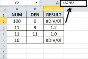
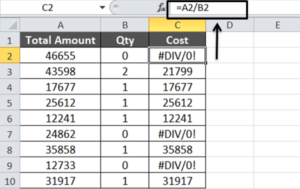
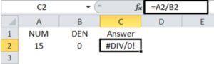
In the above picture we have taken a basic calculation of division. But you can see the formula is giving the error whenever the value is divided by 0 or space and to prevent the formula from errors, we will use the IFERROR function here.
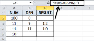
In IFERROR function the first parameter will be the formula shown in above picture and when the formula gives error then we want IFERROR function to return any other value which is value_if_error parameter. Let’s ask the IFERROR function to return the Blank cell by supplying an empty string “”.
In the above picture the formula used is:
=IFERROR(A2/B2,””)
The first parameter is the formula or calculation which to test and if the first parameter gives error then we have entered an empty string in the second parameter i.e. “” to get a blank cell.
Now instead of blank cells, we can also return the value in text or any message. Let’s see that.
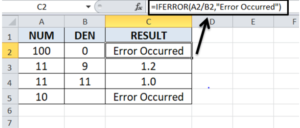
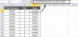
Now we have asked the IFERROR function that if the calculation or formula gives error then return the value in text as “Error Occurred”.
Isn’t this function a lifesaver while dealing with the errors and keeping the excel sheets at a user-friendly experience.😊
Let’s try to understand it with more advanced examples.
2.) IFERROR Function with VLookup
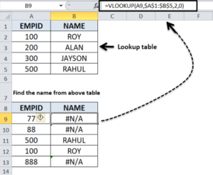
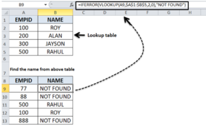
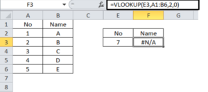
So, most of the time the VLookup function throws an error when the value we are looking for does not exist in the data set as shown in the picture below.
As we can see in second table of the above picture that while finding the Name from first table with vlookup, it has returned the #N/A value when it’s unable to find the value.
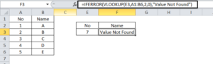
Now to prevent errors and for user -friendly experience, let’s use the IFERROR function and ask it to return us the value as “Not Found” when the VLookup function is giving error.
As we can see the IFERROR function has returned the value as “NOT FOUND” wherever the VLOOKUP function given the error.
3.) IFERROR with VLookup
Now you may have a situation where you need to perform the multiple VLookups with different tables and when the previous VLOOKUP function gives error then we can nest it with two or more IFERROR functions. Let’s see this with an example to make it more clear in our mind.
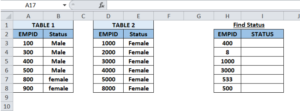
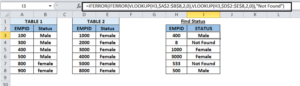
As shown in the below picture, we have two tables with employee ID and Status and In third table, we have to find the status of employee ID from two tables. So, just to understand it easily, I have kept the tables close to each other in one sheet but you may have a situation where the table data is present in a different sheet or workbook.
Now, Let’s search the value in the first table with the VLOOKUP function.
As we can see in the above picture, the VLOOKUP function has returned the status for the values present in the 1st table. But the few lookup values are also present in the 2nd table hence we will use IFERROR function here and will ask IFERROR function that wherever the VLOOKUP function has given the error, please check the output in 2nd table for those values with VLOOKUP function.
So, let’s see what the formula will look like.
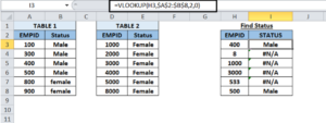
As we can see in the above picture, we have used the IFERROR function to run another VLOOKUP function. When the first VLOOKUP Function fails to find the value in 1st table, using the IFERROR function we have used another VLOOKUP function to find the values from 2nd Table.
Now, we can see there are still #N/A error for few values in the 3rd table and it’s just because the both VLOOKUP function cannot find those values from Table 1 and Table 2. So the get rid from those errors we will run another IFERROR function and we will ask IFERROR function to give the result text as “Not Found” wherever at the place of #N/A.
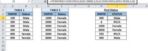
Let’s see what the formula will look like.
So, Now we can see that the IFERROR function has returned the result as “Not Found” to the values which are not present in the both given tables.
4.) ISERROR Function
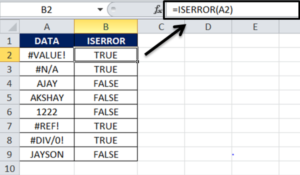
ISERROR function is the logical function which is used to check whether a cell contains the error value or not. It gives result in boolean value, If we insert any formula, calculation or value inside the ISERROR function and that returns any error then ISERROR function will give TRUE as result and when the formula, calculation or value inside the ISERROR function does not returns any error or run successfully then ISERROR function will return FALSE as result.
Syntax of ISERROR function simple:
=IFERROR(Value)
Let’s see the example to understand it better.
As we can see in the above picture, when the cell contains any error value the ISERROR function has returned the TRUE as result and when the cell does not contain any error the result returned is FALSE.
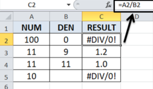
Let’s see another example on the basis of calculation.
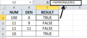
In the above picture, we have taken a simple calculation of division and it has returned an error when the numerator is divided by 0 or space. Let’s use the ISERROR function here and see how that will look like.
So we can see in the above picture that the IFERROR function has returned the TRUE when the calculation given the error.
The IFERROR function is easy to identify the error and gives the result as TRUE whenever the error occurred. But what if you want to return any text value or custom message or run formula instead of Boolean value as TRUE and FALSE. Now, the IF and ISERROR function works better here.
Let’s understand the IF and ISERROR combination in the next topic.
5.) IF Function with ISERROR (wow wow):
Now, By using the IF function and ISERROR function combined, it can help to return any text, custom message and calculation when the error occurs.
In simple words when the ISERROR function identifies an error then the IF function will run any custom message, text value or another calculation or it will run the main calculation as it is.
Let’s see an example to clear it in our mind.
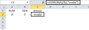
In the above picture, we have taken a simple calculation of division and when the amount is divided by 0, the calculation returned error as #DIV/0!.Now let’s use the IF Function with ISERROR function to return the text value as “Invalid” instead of errors and see how the formula will look like.
So in the above picture, we have used the IF and ISERROR function combined and when the calculation inside the ISERROR function returns an error the IF function returns the “Invalid” as text message and otherwise it returns the calculation.
Now I hope that we must be clear with IF and ISERROR functions. The IF ISERROR function performs results similar to the IFERROR function and both functions are used for error detection and error prevention.
Lets see the difference between IFERROR and IS IFERROR function.
6.) IFERROR vs IF ISERROR function :
Now you must be wondering if the IFERROR function and IF ISERROR function gives similar results then are there any advantages of IF ISERROR function. Well NO..
In older versions of Excel 2003 and before when the IFERROR function did not exist. The IF ISERROR function was the only way to detect the errors and prevent the excel formula from errors.
Lets see the difference between the IFERROR and IF ISERROR function. Suppose we used the Simple division calculation and to catch the error, we used formulas as below.
IFERROR function: =IFERROR(A1/B1,”Value not found”)
IF ISERROR function: =IF(ISERROR(A1/B1),”Value not found”,A1/B1)
As we can notice in the IFERROR function, The calculation runs only one time and if it returns any error then it will return the text as “Value not found” otherwise the Calculation will run successfully.
Whereas in IF ISERROR function, The Calculation runs twice and when it gives an error then it will return text as “Value not found” , otherwise the calculation will run another time.
So, it means if i have to do two different things at a time based on error – that if error comes I will go to college and if there is no error I will go to a beach, then I will use IF(ISERROR) and on the other hand , If there is an error then i will go to a college and if there is no error then wherever I am , i will be there – you know kind of that situation ,so we use IFERROR. Both are powerful and both have their own importance. So, if i am looking for either formula result value or in case of an error looking for some other thing – IFERROR is my choice.
In my experience, I have dealt with IFERROR more often than the other one.
Hopefully, we are clear about IFERROR and IF ISERROR function. So let’s see now the Types of errors, its cause and how we can get rid of it through IFERROR function.
7.) Types of errors with example:
#N/A Error:
The N/A means “Not Available”, So when you are looking for any value in range through VLOOKUP or any other formula, and that value is not present in the range, then this error will occur.
Let’s take an example:
As you can see in the above picture, the VLOOKUP function has an error when it cannot find the value. Now, let’s use the IFERROR function and return the “Value Not Found”.
#DIV/0! Error:
This error occurs when dividing any number by 0 or equivalent to 0 that can be blank cell as well. Hence, the #DIV/0! Error occurred which shows that we are trying to divide a number by 0.
As we can see above that we have divided a number 15 by 0 and it has given the #DIV/0!.
Let’s now use the IFERROR function and bring the “Invalid” as a result.
#Name? Error:
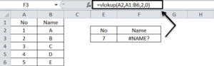
This error occurs when we enter the formula name incorrectly. Suppose we are using the VLOOKUP function but instead you have entered VLOKUP. The excel does not know what you mean due to Typo mistake and it will give the error as shown below.
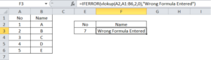
In this case we should enter the correct name of the formula to recognize it by excel and give desired results. For Now, Let’s use the IFERROR function and get the text result as “Wrong Formula Entered”.
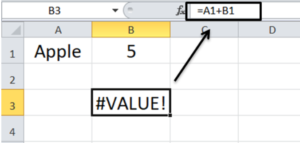
#Value! Error:
This error occurs when we have taken the incorrect value type. Suppose you want to sum two numbers from two cells but you entered the text value in the second cell hence the calculation cannot be performed as you can’t sum the text and number as shown below.
So, we have to ensure that the format of both cells are correct to get the desired results. Now, let’s use the IFERROR function and replace error by custom message “Incorrect Type”
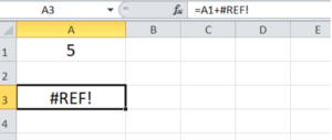
#REF! Error:
This error occurs in the excel when you enter the invalid reference in the formula or the reference column you have entered is deleted. Suppose you did sum of two cells and one of the cell column is deleted then you will get the #REF! Error as shown below.
Let’s delete column B and see.
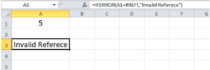
So by doing this #REF! Error occurred and to replace the error by custom massage. We can use the IFERROR function here.
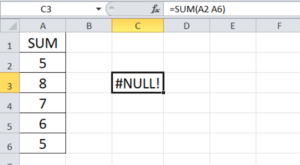
NULL! Error:
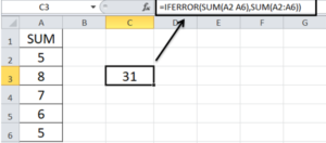
This error is rare in excel, but this error can occur in excel when the space is entered between two cell references instead of Comma ( , ) or colon(:). Lets see this with an example.
As we can see in the above picture, when we have entered space instead of colon the formula has given the error as #NULL!. Let’s use the IFERROR function and bring actual results by formula.
Hopefully, This blog may have helped you to know IFERROR and IF ISERROR function better. Thank you for reading this blog. See you soon in another blog. ❤️❤️❤️❤️❤️