Excel IF Functions -Like never Before – In depth Study

The IF function is one of the functions which is widely used in excel and makes it easy to classify the data as per the condition given. Lets go further in detail to understand the IF function and I will assure you that this blog post will help you to grasp your excel skills. 😀

Topics we have covered here :

What is the IF function and How to use it ?
IF with AND
IF with OR
Nested IF
What is the IFS function (office 365 and latest)
IFS (Office 365) vs Nested IF
IF with Case sensitive texts
IF with Partial Match
IF with Dates

1. ) What is the IF function and How to use it ?

It’s the function which checks for the condition. If the first condition is met then it returns the True value and if the second condition is met then it will return the False value. It is one of the flexible functions which helps to calculate values based on certain conditions and also to categorize the data. Lets see its syntax and the parameters.

Syntax of IF function is:

=IF(logical_test, value_if_true, value_if_false)

As we can see in the above formula, there are three parameters in the formula. The Parameters are :

logical_test : It’s the obligatory condition in order to get the result. This parameter is to test and evaluate the condition either as true or false. The condition can be evaluated using below 6 logical operators.
- Equal to (=)
- Not equal to (<>)
- Greater than (>)
- Greater than equal to (>=)
- Less than (<)
- Less than equal to (<=)

We will see these logical operators in the coming examples.

a. Value_if_true : its the value returned when the logical test evaluates to True that means the given condition is met. It’s optional but if it’s omitted, we must define the input in value_if_false criteria to get the result.

b. Value_if_false: its the value returned when the logical test evaluates to False that means the given condition is not met. It’s also optional but if it’s omitted, we must define the input in value_if_true criteria to get the result.

Let’s see an example to understand it’s syntax well.

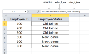
As we can see in the above example. We have the data of employee ID’s in the first column. And in another column we have to find the employee status as “Old Joinee” and “New Joinee” Also we have a condition that if employee ID is greater than 300 then the value as output should be as “New Joinee” and other should be “Old Joinee”. So, to find that we have used the IF function in B2 cell i.e. “=IF(A2>300,”New Joinee”,”Old Joinee”)”.

In the given formula, we have used first parameter as logical test is A2>300 and this to test if the value in cell A2 is greater than 300 or not, then in second parameter as value_if_true we inserted “New Joinee” because if our condition is met then we want the result as “New Joinee” and in last parameter as value_if_false we inserted “Old Joinee” because if our condition is not met i.e if the value is not greater than 300 then we want the result as “Old Joinee”. Afterwards we have drag the formula till B7 cell to find the result for all other employee ID’s

Let’s see another example to make the If function more clear in our mind.

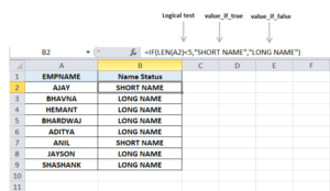
As we can see in the above example. We have the data of employee Names in the first column. And in another column we have to find the Name status as “SHORT NAME” and “LONG NAME” Also we have a condition that if length of employee name is less than 5 letters then the value in output should be as “SHORT NAME” and other should be “LONG NAME”. So, to find that we have used the IF function in B2 cell i.e. “=IF(LEN(A2)<5,”SHORT NAME”,”LONG NAME”)”.

In the given formula, we have used the first parameter as the logical test is LEN(A2)<5. Now as you see we have used the LEN function in the formula which helps to find the length of the value present in cell and this checks if the length of value in cell A2 is less than 5 or not, then in second parameter as value_if_true we inserted “SHORT NAME” if the condition is met and in last parameter as value_if_false we inserted “LONG NAME” if our condition is not met. Afterwards we drag the formula till B9 cell to find the result for all other employee Names.

Now, Hope that we are clear with the Basic If function and it’s time to deep dive more in it. We will see IF function furthermore now by using AND Function in it.

2.) IF with AND :

Now, before we use the IF & AND function combined, let’s understand what AND function is and how it can play an important role in order to get the result in multiple conditions.

AND function is a logical function which checks whether all conditions specified in the formula are TRUE. If all conditions given in the formula are met then it gives TRUE as result and if any of the conditions is not met then it gives FALSE as a result. Let’s understand it by an example.

Syntax of AND Function is :

=AND(logical1, [logical2], …)

As we can see in the above image, we have the data of Students Name and their marks in Science and English columns. And we have used the AND function in cell D2 to check whether the Marks of Science and English subjects are greater than 50 or not. Hence, we have used “=AND(B2>50,C2>50)”. First condition i.e. Logical1 is B2>50 which checks if value in cell B2 is greater than 50 or not and second condition i.e. Logical2 is C2>50 which checks if value in cell C2 is greater than 50 or not And when both given conditions are met or TRUE, then we get the result as TRUE which we can see in column D i.e. in Status.

Hope that we are clear about how AND function works. Let’s see now the IF function with AND Function to explore the magic of it. It’s a very useful function when we have more than one criteria and all of the conditions should be met.

The syntax is :

=IF(AND(logical1, [logical2],), value_if_true, value_if_false)

Let’s see this with a recent example.

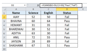
As we can see in the picture, we have the data of Name and Marks in Science and English subjects And we have to find the Pass/Fail status in column D with the condition that the marks should be more than 50 in both subjects for “Pass” status if any of subject has less than 50 marks then status should be “Fail”, hence we have used the IF function with AND function as followed:

In the above formula, we have used the AND function as a logical test i.e. AND(B2>50,C2>50) and as we have seen in the AND functions example, it checks if the value in cell B2 and C2 is greater than 50 or not. If both subjects marks are greater than 50 that means the conditions are met and as we stated “Pass” in value_if_true if both conditions met and we stated “Fail” in value_if_false, if any or none of the conditions is not met. So in cell D2 to D9 we can see the results received as per the conditions. Isn’t it useful to classify the data as per the conditions.

Let’s turn towards our next topic to reveal the power of IF function more. We will now see IF and OR function combined when we want any given condition to be met.

3.) IF with OR :

Let’s first understand the OR function before we combine it with the IF Function. The OR function is a logical function which allows us to test the multiple conditions and It returns TRUE if any of the one specified condition is met and it returns False when all the conditions are not met.

Now we have seen AND function in the above topic and also we are covering OR function in this Topic. So the only difference between these both functions is AND function needs all conditions to be met to get TRUE result and OR function needs any of the given conditions to be met to get TRUE result.

Syntax of OR function :

=OR(logical1, [logical2], …)

Lets see an example of OR function.

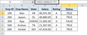
As we can see in the above image, we have the data of Emp ID, Emp Name, State, Salary and the Rating. We have to check if Employee’s salary is greater than 40,000 or Employees Rating is equal to A or not. As we want any one of the condition to be met hence we have used the OR function i.e. =OR(D2>40000,E2=”A”). In the formula, the first condition is D2>40000 which checks if the value in cell D2 is greater than 40,000 or not. And the second condition is E2=”A” which checks whether the value in E2 cell is equal to A or not. So when any of the conditions is met then Output in cell F2 comes as TRUE which we can see in the above shown image and the formula is dragged down to get results for other rows.

Now hope that we are clear about how the OR function works and lets see the IF function with OR function in multiple conditions ahead.

Syntax of IF function with OR function :

IF(OR(logical1, [logical2],), value_if_true, value_if_false)

Lets understand with the recent example:

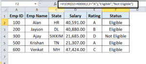
As we can see in the picture, we have the same data set used in earlier example but now in F2 cell we have combined the IF and OR function as followed:

In above given formula, As logical test we have used OR function i.e. OR(D2>40000,E2=”A”) and in the OR function we have stated two conditions. First condition is to check whether value in cell D2 is greater than 40,000 or not and the Second condition checks whether value in cell F2 is equals to “A” or not and any of the these two condition is met then we will get the result from value_if_true which is “Eligible” and if no any condition is met then we will get the result from value_if_false which is “Not Eligible”. As we can see in the F column the formula has given the output accordingly.

4.) Nested IF function:

Let’s be excited about another smashing topic of IF function. Nested IF function is nothing but using the IF function multiple times inside of the IF function itself. As a basic IF function can test the one condition but what if we have multiple conditions, in this case we have to include multiple IF functions in one formula and this nesting creates the Nested IF function.

Syntax of Nested IF Function:

=IF(logical_test1, value_if_true1, IF(logical_test2, value_if_true2, value_if_false2))

Lest see its example and understand it well.

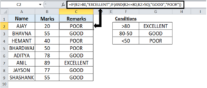
As we can see in the above picture, we have the data of Students Name and Marks and the conditions given are : EXCELLENT : >80 Marks, GOOD : 80-50 Marks , POOR : <50 Marks. And We have used the IF function in cell C2 as followed:

=IF(B2>80,”EXCELLENT”,IF(AND(B2<=80,B2>50),”GOOD”,”POOR”))

So, it’s a good practice to use the conditions in order to get the correct result as we used in the above formula. Let’s try to see the above formula from a different angle .

What the formula actually says is to evaluate the logical_test of the first IF function and if the condition is met, then return the value supplied in the value_if_true argument. If the condition of the 1st If function is not met, then test the 2nd If statement.

The first IF condition is B2>80 which checks whether value in cell B2 is greater than 80 or not. If the first condition is met then it will return value_if_true which is “EXCELLENT” and if the condition is not met then it will test another logical test in IF function which is AND(B2<=80,B2>50). This checks whether the value in the cell B2 is greater than 50 and Less than equals to 80 or not and if both the given conditions are met then it will return the value_if_true which is “GOOD”. If none of the given previous conditions are met then it will return the value_if_false which is “POOR”. In the C column the result is shown with the Nested IF function.

5.) What is the IFS function and How to use it?

As we have seen the Nested IF function in the last topic, the IFS function is an alternative function to the Nested IF and It’s very easy to use as well. The IFS function allows you to test the multiple conditions and when the first true condition is met then it results corresponding true result. This function was introduced in 2016 and you can test up to 127 conditions in it which makes it more powerful.

Let’s see its Syntax and examples to understand it well.

Syntax of IFS function: =IFS(logical_test1, value_if_true1, [logical_test2, value_if_true2], …logical_test127, value_if_true127)

In the above formula, logical_test 1 is a required argument and it is a condition which is used to evaluate as TRUE or False and Value_if_true1 is the result when the first logical test is true. Rest logical test and Value arguments are optional and you can enter up to 127 logical test arguments. But only downside of this function is you can’t give Else condition as formula dont have option. But we can sort this issue as well which we will see in upcoming examples

Let’s see the example now.

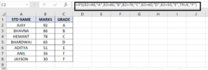
As we can see in the above image, we have the data of the student name with marks and in column C the Grade should be retrieved. We have entered the conditions and when the given condition is met the value is retrieved accordingly in column C as grade.

The formula used is :

=IFS(B2>90,”A”,B2>80,”B”,B2>70,”C”,B2>60,”D”,B2>50,”E”,TRUE,”F”)

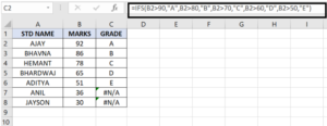
In the above formula we have given the condition till 50 but what if the table contains values less than 50. The result will look like this.

The result which IFS function returned for values less 50 is #N/A because we have not specified any condition for it and the IFS function dont have the option of ELSE to specify it. But we can ensures this #N/A error is removed and for this we would place a final test at the end of the formula which is TRUE and then place a value which we want to be returned.

As we can see in the above image we have added TRUE , “F” at the end and this will ensure that the function will return the value “F” when none of the conditions is met.

6.) IFS Function vs Nested IF :

As we have covered the Nested IF function Topic before IFS functions Topic. So let’s see by using these two functions for the same example and find out which function is easy to use.

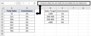
Let’s assume that we have the data of employee sales and we want to give them a commission based on sales count. So, sales made less than 200 will get 1% commission, a 2% commission for sales more than 200 and less than 500. a 3% commission for sales more than 500 and less than 800 and a 4% commission on sales made more than 800.

Lets see the formula using Nested IF Function:

Now let’s see how easy it is to write IFS formula to bring similar results:

As you can see in the first image of the Nested IF function, we have entered the IF formula for every condition which we have given and In the second image of IFS function we have entered many conditions in a single function which makes IF function easier than nested IF function. Hence IFS function can be very easy and useful to operate while in multiple conditions.

Now, By reading this blog post till here you are ready to go and hit the excel sheet and try applying it in your data which will help you to increase your productivity and share few insights with your boss.😜

7.) IF with Case sensitive Texts:

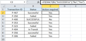
Suppose you have the data of the same texts but in Uppercase and Lowercase. In this condition we can combine IF function with Exact function. Lets see this with an example

In the above example, we have used the IF function to return “No” only when column B contains “SUCCESSFUL” (In Uppercase”).

8. ) IF (Partial match):

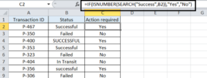
Suppose you have a situation where you want to base a condition on partial match and here the ISNUMBER and Search function can help to get the result. Let’s see how?

In the above picture, SEARCH function is used to find the word into the cell B2 which gives a text position in the cell by number and ISNUMBER function checks if the selected cell is in the number format or not and wherever SEARCH function find “Success” text in column B then it gives a number of position of that text and ISNUMBER gives true as result whenever it has find the text.

9.) IF with Dates:

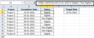
As we cannot supply a date in the form of “1/1/2023” as IF function considers it as text string and we won’t get the correct output which we want. But to make IF function recognize a date we can use the DATEVALUE function as shown in the image below.

In the above picture we have the Target date in cell E1 for the completion of the project and we have used the IF function in column C to find which project completed on and before the target date. “Eligible” For True match which is value_if_true and “Not Eligible” For False match which is value_if_false.

To run another formula:

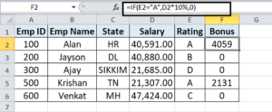
As we have seen in previous examples, the IF function returned the values. But, it can also return a calculation or any formula when the condition is met or not met. Lets see this with an example.

As we can see in the above image, to calculate the 10% Bonus on salary for someone who has a rating as “A”. we have used IF function and when the condition is met, we have inserted a calculation or formula which is D2*10% which calculates bonus and when the condition is not met then employee will not the get the bonus,

Hopefully, This blog may have helped you to know IF function better. I got to go to gym now! My headphones are looking at me and saying, we need you. Thank you for reading this blog. See you soon in another blog. Remember, if you are fit,you are hit. Health creates wealth and not vice -versa.